---
title: "Describtion"
toc: true
toc-location: left
code-fold: true
warning: false
code-tools: true
---
# 总体描述性统计
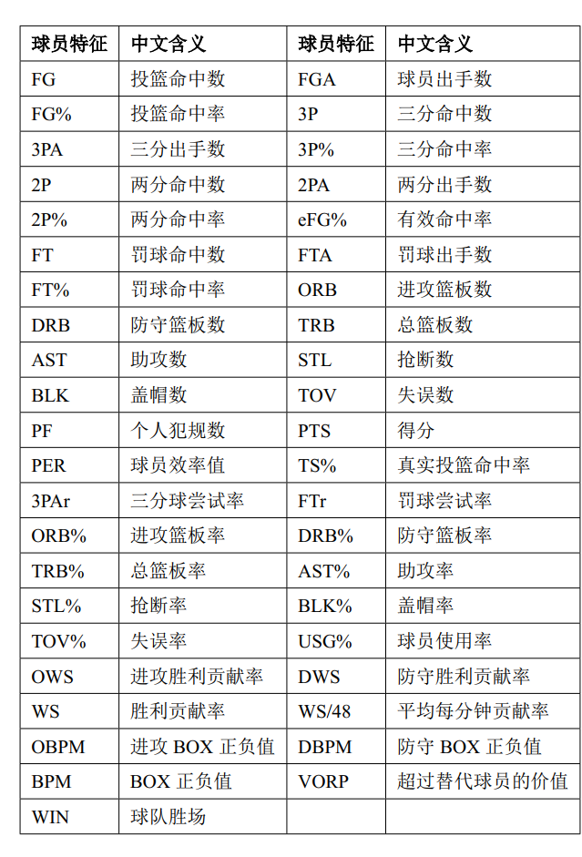
## 所用球员特征表:
```{r}
# 安装并加载所需包(如未安装请取消注释下面行)
# install.packages("readxl")
# install.packages("dplyr")

library(readxl)
library(dplyr)

# 读取 Excel 文件
df <- read_excel("C:/Users/86133/Desktop/object/MVP/常规赛.xlsx")

# 查看列名和前几行
names(df)
head(df)
# 去掉非数值列(如名字、赛季),只保留数值型列
numeric_df <- df %>%
  select(where(is.numeric))

# 基本描述性统计
summary(numeric_df)
# 计算均值、标准差、最小值、最大值等更全面的统计量
```
```{r}
# 安装必要包(首次运行时需要)
#install.packages("gt")
library(dplyr)
library(tidyr)
library(gt)

# 计算全面统计量(宽数据格式)
stat_wide <- numeric_df %>%
  summarise_all(
    list(
      mean = ~mean(.x, na.rm = TRUE),
      sd = ~sd(.x, na.rm = TRUE),
      min = ~min(.x, na.rm = TRUE),
      q1 = ~quantile(.x, 0.25, na.rm = TRUE),
      median = ~median(.x, na.rm = TRUE),
      q3 = ~quantile(.x, 0.75, na.rm = TRUE),
      max = ~max(.x, na.rm = TRUE)
    )
  )

# 转换为长数据(变量与统计量分离)
stat_long <- stat_wide %>%
  pivot_longer(
    cols = everything(),
    names_to = c("variable", "statistic"),  # 拆分为变量名和统计量名
    names_sep = "_"                         # 列名通过下划线分割(如"mpg_mean" → "mpg"和"mean")
  )

# 转换为宽数据(统计量作为列,变量作为行),并保留variable列
stat_table <- stat_long %>%
  pivot_wider(
    names_from = statistic,       # 统计量名称作为列名
    values_from = value           # 统计量值作为列内容
  ) %>%
  select(
    variable,                     # 显式保留variable列(关键修正!)
    starts_with("mean"),
    starts_with("sd"),
    starts_with("min"),
    starts_with("q1"),
    starts_with("median"),
    starts_with("q3"),
    starts_with("max")
  )  # 按顺序排列列(可选)

# 用gt绘制表格(此时stat_table包含variable列)
stat_table %>%
  gt() %>%
  tab_header(
    title = "数值变量的描述性统计量",
    subtitle = "包含均值、标准差、分位数等"
  ) %>%
  cols_label(
    variable = "变量",  # 现在variable列存在,不会报错
    mean = "均值",
    sd = "标准差",
    min = "最小值",
    q1 = "第一四分位数 (25%)",
    median = "中位数",
    q3 = "第三四分位数 (75%)",
    max = "最大值"
  ) %>%
  fmt_number(
    columns = everything(),
    decimals = 2
  ) %>%
  tab_style(
    style = cell_text(weight = "bold"),
    locations = cells_title(groups = "title")
  ) %>%
  tab_options(
    column_labels.font.weight = "bold",
    table.font.size = 12,
    data_row.padding = px(8)
  )
```
```{r}
library(readxl)
library(dplyr)
# 总样本量(原始数据行数)
total_rows <- nrow(df)

# 每列的缺失值个数
missing_per_column <- colSums(is.na(df))

# 缺失值总数
total_missing <- sum(is.na(df))

# 删除所有含有缺失值的行
df_no_na <- df %>% drop_na()

# 删除后剩余的行数
remaining_rows <- nrow(df_no_na)

# 被删除的行数
removed_rows <- total_rows - remaining_rows

# 汇总信息为表格
summary_table <- data.frame(
  指标 = c("总样本量", "含缺失值的样本量", "删除后剩余样本量", "缺失值总个数","指标总数"),
  数值 = c(total_rows, removed_rows, remaining_rows, total_missing,43)
)

print(summary_table)
```
## 指标随赛季变化折线图
```{r}
library(readxl)
library(dplyr)
library(tidyr)
library(ggplot2)

df <- read_excel("C:/Users/86133/Desktop/object/MVP/常规赛.xlsx")

# ---------------------------
# 步骤1:处理常数列并归一化(避免NaN)
# ---------------------------
# 选择数值列并识别常数列(max == min)
numeric_cols <- df %>% select(where(is.numeric)) %>% colnames()
constant_cols <- sapply(df[numeric_cols], function(col) {
  isTRUE(all.equal(min(col, na.rm = TRUE), max(col, na.rm = TRUE)))
})

# 仅对非常数列进行归一化,常数列设为0(或根据需求处理)
df_scaled <- df %>%
  mutate(
    across(
      all_of(numeric_cols[!constant_cols]),  # 仅处理非常数列
      ~ (. - min(., na.rm = TRUE)) / (max(., na.rm = TRUE) - min(., na.rm = TRUE))
    ),
    across(
      all_of(numeric_cols[constant_cols]),  # 常数列设为0(或其他合理值)
      ~ 0
    ),
    Season = df$Season  # 添加赛季列
  ) %>%
  select(Season, all_of(numeric_cols))  # 整理列顺序(可选)

# ---------------------------
# 步骤2:计算各赛季均值(处理全NA情况)
# ---------------------------
mean_by_season <- df_scaled %>%
  group_by(Season) %>%
  summarise(
    across(where(is.numeric),
           ~ ifelse(sum(is.na(.)) == length(.),  # 检查是否全为NA
                    NA_real_,                # 全NA则返回NA
                    mean(., na.rm = TRUE))),   # 否则计算均值
    .groups = "drop"
  )

# ---------------------------
# 步骤3:转换为长格式并整理
# ---------------------------
mean_long <- mean_by_season %>%
  pivot_longer(
    cols = -Season,
    names_to = "Variable",
    values_to = "Mean"
  ) %>%
  mutate(
    Season = factor(Season, levels = sort(unique(Season))),  # 控制赛季顺序
    Variable = factor(Variable)  # 确保变量为因子,正确分组
  ) %>%
  filter(!is.na(Mean))  # 移除均值中的NA(可选,根据需求保留)
```
```{r}
library(ggplot2)
library(dplyr)
library(patchwork)  # 用于图拼接

# 步骤1:变量分组
variables <- unique(mean_long$Variable)
n_vars <- length(variables)
group_size <- 5
group_ids <- ceiling(seq_len(n_vars) / group_size)
Group <- paste0("Group_", group_ids)
variable_group_map <- data.frame(Variable = variables, Group = Group)

mean_long_grouped <- mean_long %>%
  left_join(variable_group_map, by = "Variable")

# 步骤2:为每个 group 生成一个图(含图例)
plots <- list()

groups <- unique(mean_long_grouped$Group)

for (g in groups) {
  df_sub <- mean_long_grouped %>% filter(Group == g)

  p <- ggplot(df_sub, aes(x = Season, y = Mean, color = Variable, group = Variable)) +
    geom_line(size = 0.7, alpha = 0.5) +
    theme_minimal(base_size = 8) +
    theme(
      axis.text.x = element_text(angle = 90, hjust = 1, size = 4),
      axis.text.y = element_text(size = 4),
      strip.text = element_text(size = 5, face = "bold"),
      legend.position = "top",
      legend.text = element_text(size = 5),
      legend.title = element_blank(),
      plot.title = element_text(size = 5, face = "bold"),

    ) +
    labs(
      title = paste("归一化变量均值变化 -", g),
      x = "赛季",
      y = "归一化均值"
    )

  plots[[g]] <- p
}

# 步骤3:拼接所有图(2列排列)
final_plot <- wrap_plots(plots, ncol = 3)
final_plot
#ggsave("grouped_plots.png", final_plot, width = 15, height = 10, dpi = 500)
```
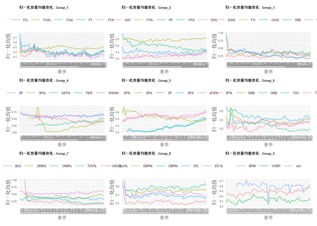
1.上世纪50年代,总投篮出手次数逐渐减少而后趋于稳定,而命中率上升,可能表示技术精进、精细,团队合作
2.上世纪80-90年代,命中率(主要是两分球)达到峰值后90-2000又下降(可能是防守强度上升),后又逐渐上升(技术精进)
3.三分球占总投篮比例(3PAr)在1966年达到峰值后下降到73年逐步上升至今(幅度很大)
4.三分球出手数稳步提升于2017年超过两分球,同时三分球,两分球等投篮命中率在2000年后稳步提升
5.ORB(进攻篮板)逐年下降趋势(下降明显),AST助攻近年逐步上升
6.PF犯规逐年递减
# 总体和MVP对比柱状图
赛季均值数据:
```{r}
# 加载所需的包
library(readxl)
library(dplyr)
library(writexl)
#install.packages("writexl")
# 读取 Excel 文件
data <- read_excel("C:/Users/86133/Desktop/object/MVP/常规赛.xlsx")


# 假设年份列为 "Season",对其分组并求每列的均值
mean_by_year <- data %>%
  group_by(Season) %>%
  summarise(across(where(is.numeric), mean, na.rm = TRUE))

# 保存为新的 Excel 文件
write_xlsx(mean_by_year, path = "C:/Users/86133/Desktop/object/MVP/每年均值.xlsx")
```
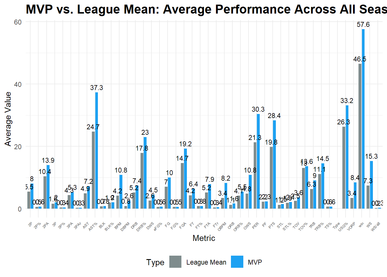
## 2010-2023赛季 MVP 和 总体数据 对比柱状图:
```{r}
#| warning: false
library(readxl)
library(dplyr)
library(tidyr)
library(ggplot2)
library(stringr)

# 读取数据
df <- read_excel("C:/Users/86133/Desktop/object/MVP/MVP_Mean/MVP_mean_2010_23.xlsx", sheet = "Sheet1")

# 提取年份和类型
df <- df %>%
  mutate(
    Season = str_extract(name, "\\d{4}"),
    Type = ifelse(grepl("Mean", name), "League Mean", "MVP")
  )

# 分别计算平均值(跨所有赛季)
mvp_mean <- df %>%
  filter(Type == "MVP") %>%
  select(-name, -Season) %>%
  summarise(across(everything(), mean, na.rm = TRUE)) %>%
  pivot_longer(cols = everything(), names_to = "Metric", values_to = "Value") %>%
  mutate(Type = "MVP")

league_mean <- df %>%
  filter(Type == "League Mean") %>%
  select(-name, -Season) %>%
  summarise(across(everything(), mean, na.rm = TRUE)) %>%
  pivot_longer(cols = everything(), names_to = "Metric", values_to = "Value") %>%
  mutate(Type = "League Mean")

# 合并
compare_df <- bind_rows(mvp_mean, league_mean)

# 绘图
ggplot(compare_df, aes(x = Metric, y = Value, fill = Type)) +
  geom_col(position = position_dodge(width = 0.8), width = 0.7) +
  geom_text(
    aes(label = round(Value, 1)),
    position = position_dodge(width = 0.8),
    vjust = -0.5,
    size = 3
  ) +
  scale_fill_manual(values = c("MVP" = "#1DA1F2", "League Mean" = "#7F8C8D")) +
  labs(
    title = "MVP vs. League Mean: Average Performance Across All Seasons",
    x = "Metric",
    y = "Average Value",
    fill = "Type"
  ) +
  theme_minimal() +
  theme(
    axis.text.x = element_text(angle = 45, hjust = 1,size=5),
    plot.title = element_text(size = 16, face = "bold"),
    legend.position = "bottom"
  )
```
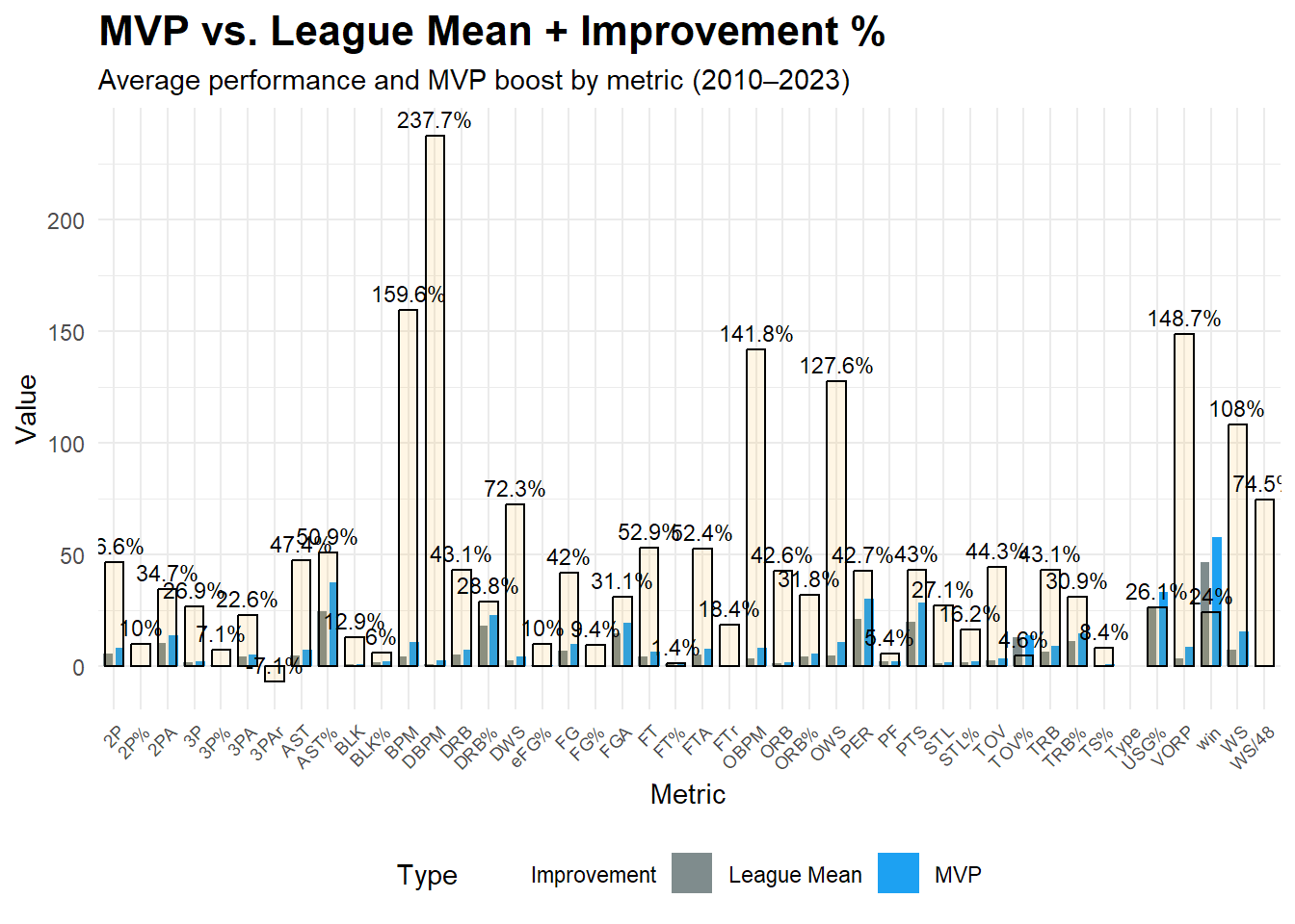
2010-2023赛季 MVP 和 总体数据 对比柱状图:
```{r}
#| warning: false
# 将 MVP 和 League Mean 数据展开为宽格式
df_wide <- compare_df %>%
  pivot_wider(names_from = Type, values_from = Value)

# 计算提升百分比(%),并构建新数据框
improvement_df <- df_wide %>%
  mutate(`Improvement %` = (`MVP` - `League Mean`) / `League Mean` * 100) %>%
  select(Metric, `Improvement %`) %>%
  mutate(Type = "Improvement") %>%
  rename(Value = `Improvement %`)

compare_all <- bind_rows(compare_df, improvement_df)

library(ggplot2)

ggplot(compare_all, aes(x = Metric, y = Value, fill = Type)) +
  geom_col(
    data = subset(compare_all, Type != "Improvement"),
    position = position_dodge(width = 0.9),
    width = 0.7
  ) +
  geom_col(
    data = subset(compare_all, Type == "Improvement"),
    aes(fill = "Improvement"),
    position = position_dodge(width = 0.9),
    width = 0.7,
    color = "black",
    fill = "orange",
    alpha = 0.1
  ) +
  geom_text(
    data = subset(compare_all, Type == "Improvement"),
    aes(label = paste0(round(Value, 1), "%")),
    vjust = -0.5,
    size = 3,
    position = position_dodge(width = 0.9)
  ) +
  scale_fill_manual(
    values = c("Improvement" = "orange","MVP" = "#1DA1F2", "League Mean" = "#7F8C8D")
  ) +
  labs(
    title = "MVP vs. League Mean + Improvement %",
    subtitle = "Average performance and MVP boost by metric (2010–2023)",
    x = "Metric",
    y = "Value",
    fill = "Type"
  ) +
  theme_minimal() +
  theme(
    axis.text.x = element_text(angle = 45, hjust = 1,size=7),
    plot.title = element_text(size = 16, face = "bold"),
    legend.position = "bottom"
  )
```
1. **3PAr**(三分出手率(3PA / FGA),三分出手占总投篮的比例) 数据低于均值
2. 提升幅度最高的几项指标:**DBPM** 防守 Box Plus/Minus衡量球员对球队进攻影响, **BPM** 综合 Box Plus/Minus(越大越好), **VORP** 替代值胜利(Value Over Replacement Player),表示比替补平均水平好多少, **OBPM** 进攻 Box Plus/Minus(衡量球员对球队进攻影响), **OWS** 进攻 Box Plus/Minus(衡量球员对球队进攻影响), **DWS** 防守胜利贡献值(Defensive Win Shares), **WS** 总胜利贡献值(Win Shares)
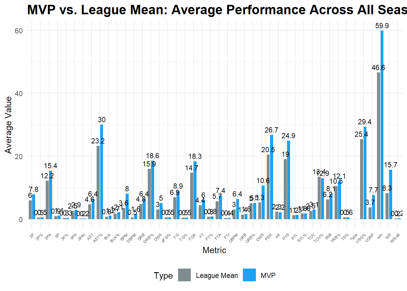
## 2000-2009赛季:
```{r}
library(readxl)
library(dplyr)
library(tidyr)
library(ggplot2)
library(stringr)

# 读取数据
df <- read_excel("C:/Users/86133/Desktop/object/MVP/MVP_Mean/MVP_mean_2000_09.xlsx", sheet = "Sheet1")

# 提取年份和类型
df <- df %>%
  mutate(
    Season = str_extract(name, "\\d{4}"),
    Type = ifelse(grepl("Mean", name), "League Mean", "MVP")
  )

# 分别计算平均值(跨所有赛季)
mvp_mean <- df %>%
  filter(Type == "MVP") %>%
  select(-name, -Season) %>%
  summarise(across(everything(), mean, na.rm = TRUE)) %>%
  pivot_longer(cols = everything(), names_to = "Metric", values_to = "Value") %>%
  mutate(Type = "MVP")

league_mean <- df %>%
  filter(Type == "League Mean") %>%
  select(-name, -Season) %>%
  summarise(across(everything(), mean, na.rm = TRUE)) %>%
  pivot_longer(cols = everything(), names_to = "Metric", values_to = "Value") %>%
  mutate(Type = "League Mean")

# 合并
compare_df <- bind_rows(mvp_mean, league_mean)

# 绘图
ggplot(compare_df, aes(x = Metric, y = Value, fill = Type)) +
  geom_col(position = position_dodge(width = 0.8), width = 0.7) +
  geom_text(
    aes(label = round(Value, 1)),
    position = position_dodge(width = 0.8),
    vjust = -0.5,
    size = 3
  ) +
  scale_fill_manual(values = c("MVP" = "#1DA1F2", "League Mean" = "#7F8C8D")) +
  labs(
    title = "MVP vs. League Mean: Average Performance Across All Seasons",
    x = "Metric",
    y = "Average Value",
    fill = "Type"
  ) +
  theme_minimal() +
  theme(
    axis.text.x = element_text(angle = 45, hjust = 1,size=5),
    plot.title = element_text(size = 16, face = "bold"),
    legend.position = "bottom"
  )
```
```{r}
#| warning: false
#| # 读取数据
df <- read_excel("C:/Users/86133/Desktop/object/MVP/MVP_Mean/MVP_mean_2000_09.xlsx", sheet = "Sheet1")

# 提取年份和类型
df <- df %>%
  mutate(
    Season = str_extract(name, "\\d{4}"),
    Type = ifelse(grepl("Mean", name), "League Mean", "MVP")
  )

# 分别计算平均值(跨所有赛季)
mvp_mean <- df %>%
  filter(Type == "MVP") %>%
  select(-name, -Season) %>%
  summarise(across(everything(), mean, na.rm = TRUE)) %>%
  pivot_longer(cols = everything(), names_to = "Metric", values_to = "Value") %>%
  mutate(Type = "MVP")

league_mean <- df %>%
  filter(Type == "League Mean") %>%
  select(-name, -Season) %>%
  summarise(across(everything(), mean, na.rm = TRUE)) %>%
  pivot_longer(cols = everything(), names_to = "Metric", values_to = "Value") %>%
  mutate(Type = "League Mean")

# 合并
compare_df <- bind_rows(mvp_mean, league_mean)
# 将 MVP 和 League Mean 数据展开为宽格式
df_wide <- compare_df %>%
  pivot_wider(names_from = Type, values_from = Value)

# 计算提升百分比(%),并构建新数据框
improvement_df <- df_wide %>%
  mutate(`Improvement %` = (`MVP` - `League Mean`) / `League Mean` * 100) %>%
  select(Metric, `Improvement %`) %>%
  mutate(Type = "Improvement") %>%
  rename(Value = `Improvement %`)

compare_all <- bind_rows(compare_df, improvement_df)

library(ggplot2)

ggplot(compare_all, aes(x = Metric, y = Value, fill = Type)) +
  geom_col(
    data = subset(compare_all, Type != "Improvement"),
    position = position_dodge(width = 0.9),
    width = 0.7
  ) +
  geom_col(
    data = subset(compare_all, Type == "Improvement"),
    aes(fill = "Improvement"),
    position = position_dodge(width = 0.9),
    width = 0.7,
    color = "black",
    fill = "orange",
    alpha = 0.1
  ) +
  geom_text(
    data = subset(compare_all, Type == "Improvement"),
    aes(label = paste0(round(Value, 1), "%")),
    vjust = -0.5,
    size = 3,
    position = position_dodge(width = 0.9)
  ) +
  scale_fill_manual(
    values = c("Improvement" = "orange","MVP" = "#1DA1F2", "League Mean" = "#7F8C8D")
  ) +
  labs(
    title = "MVP vs. League Mean + Improvement %",
    subtitle = "Average performance and MVP boost by metric (2000–2009)",
    x = "Metric",
    y = "Value",
    fill = "Type"
  ) +
  theme_minimal() +
  theme(
    axis.text.x = element_text(angle = 45, hjust = 1,size=7),
    plot.title = element_text(size = 16, face = "bold"),
    legend.position = "bottom"
  )
```
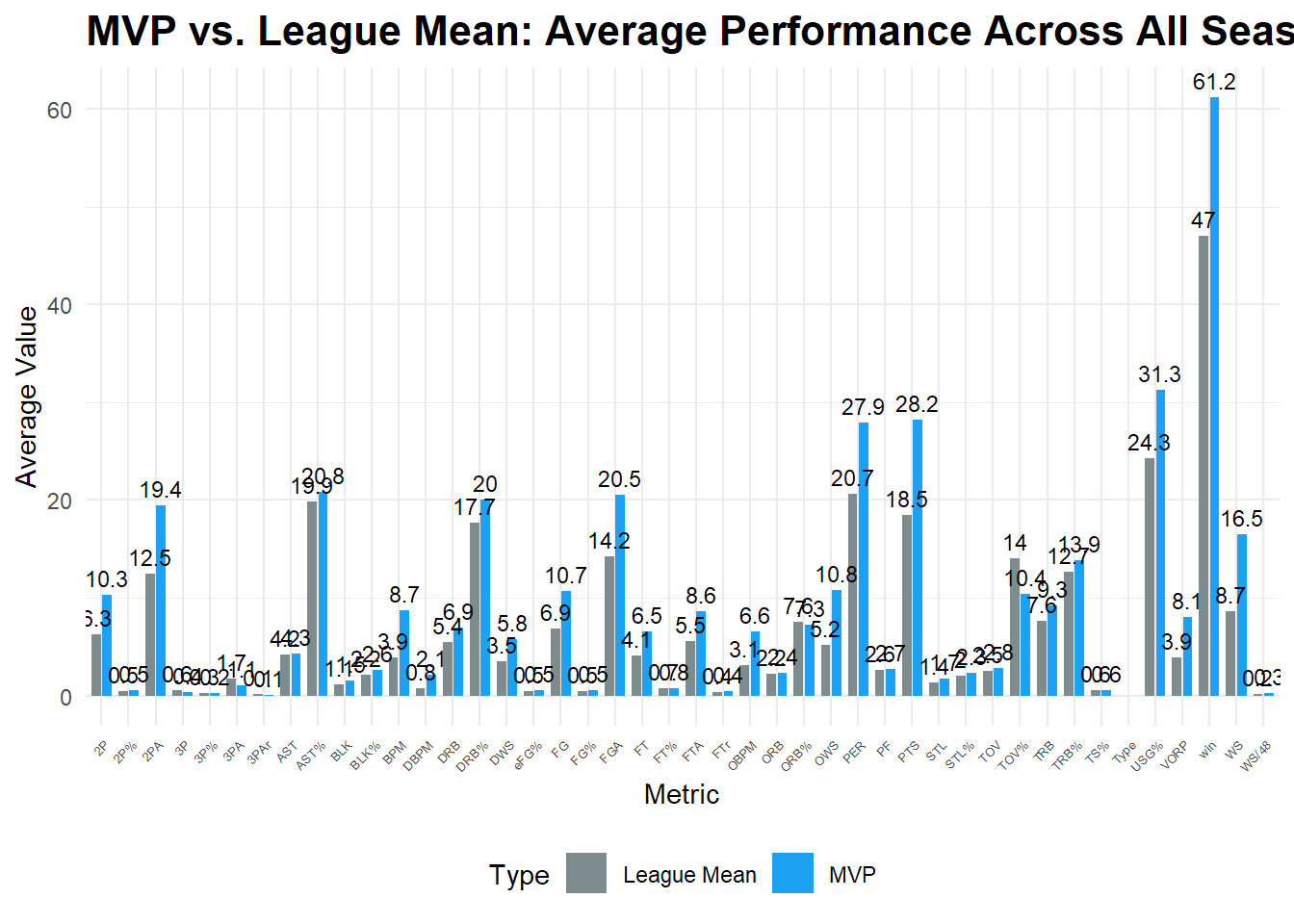
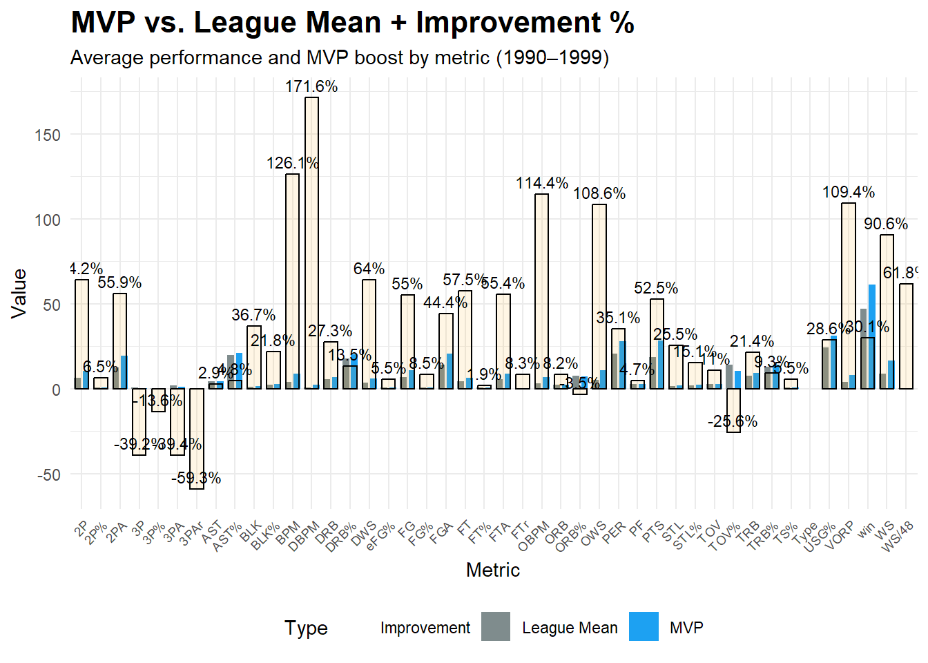
## 1990-1999赛季:
```{r}
library(readxl)
library(dplyr)
library(tidyr)
library(ggplot2)
library(stringr)

# 读取数据
df <- read_excel("C:/Users/86133/Desktop/object/MVP/MVP_Mean/MVP_mean_1990_99.xlsx", sheet = "Sheet1")

# 提取年份和类型
df <- df %>%
  mutate(
    Season = str_extract(name, "\\d{4}"),
    Type = ifelse(grepl("Mean", name), "League Mean", "MVP")
  )

# 分别计算平均值(跨所有赛季)
mvp_mean <- df %>%
  filter(Type == "MVP") %>%
  select(-name, -Season) %>%
  summarise(across(everything(), mean, na.rm = TRUE)) %>%
  pivot_longer(cols = everything(), names_to = "Metric", values_to = "Value") %>%
  mutate(Type = "MVP")

league_mean <- df %>%
  filter(Type == "League Mean") %>%
  select(-name, -Season) %>%
  summarise(across(everything(), mean, na.rm = TRUE)) %>%
  pivot_longer(cols = everything(), names_to = "Metric", values_to = "Value") %>%
  mutate(Type = "League Mean")

# 合并
compare_df <- bind_rows(mvp_mean, league_mean)

# 绘图
ggplot(compare_df, aes(x = Metric, y = Value, fill = Type)) +
  geom_col(position = position_dodge(width = 0.8), width = 0.7) +
  geom_text(
    aes(label = round(Value, 1)),
    position = position_dodge(width = 0.8),
    vjust = -0.5,
    size = 3
  ) +
  scale_fill_manual(values = c("MVP" = "#1DA1F2", "League Mean" = "#7F8C8D")) +
  labs(
    title = "MVP vs. League Mean: Average Performance Across All Seasons",
    x = "Metric",
    y = "Average Value",
    fill = "Type"
  ) +
  theme_minimal() +
  theme(
    axis.text.x = element_text(angle = 45, hjust = 1,size=5),
    plot.title = element_text(size = 16, face = "bold"),
    legend.position = "bottom"
  )
```
```{r}
#| warning: false
#| # 读取数据
df <- read_excel("C:/Users/86133/Desktop/object/MVP/MVP_Mean/MVP_mean_1990_99.xlsx", sheet = "Sheet1")

# 提取年份和类型
df <- df %>%
  mutate(
    Season = str_extract(name, "\\d{4}"),
    Type = ifelse(grepl("Mean", name), "League Mean", "MVP")
  )

# 分别计算平均值(跨所有赛季)
mvp_mean <- df %>%
  filter(Type == "MVP") %>%
  select(-name, -Season) %>%
  summarise(across(everything(), mean, na.rm = TRUE)) %>%
  pivot_longer(cols = everything(), names_to = "Metric", values_to = "Value") %>%
  mutate(Type = "MVP")

league_mean <- df %>%
  filter(Type == "League Mean") %>%
  select(-name, -Season) %>%
  summarise(across(everything(), mean, na.rm = TRUE)) %>%
  pivot_longer(cols = everything(), names_to = "Metric", values_to = "Value") %>%
  mutate(Type = "League Mean")

# 合并
compare_df <- bind_rows(mvp_mean, league_mean)
# 将 MVP 和 League Mean 数据展开为宽格式
df_wide <- compare_df %>%
  pivot_wider(names_from = Type, values_from = Value)

# 计算提升百分比(%),并构建新数据框
improvement_df <- df_wide %>%
  mutate(`Improvement %` = (`MVP` - `League Mean`) / `League Mean` * 100) %>%
  select(Metric, `Improvement %`) %>%
  mutate(Type = "Improvement") %>%
  rename(Value = `Improvement %`)

compare_all <- bind_rows(compare_df, improvement_df)

library(ggplot2)

ggplot(compare_all, aes(x = Metric, y = Value, fill = Type)) +
  geom_col(
    data = subset(compare_all, Type != "Improvement"),
    position = position_dodge(width = 0.9),
    width = 0.7
  ) +
  geom_col(
    data = subset(compare_all, Type == "Improvement"),
    aes(fill = "Improvement"),
    position = position_dodge(width = 0.9),
    width = 0.7,
    color = "black",
    fill = "orange",
    alpha = 0.1
  ) +
  geom_text(
    data = subset(compare_all, Type == "Improvement"),
    aes(label = paste0(round(Value, 1), "%")),
    vjust = -0.5,
    size = 3,
    position = position_dodge(width = 0.9)
  ) +
  scale_fill_manual(
    values = c("Improvement" = "orange","MVP" = "#1DA1F2", "League Mean" = "#7F8C8D")
  ) +
  labs(
    title = "MVP vs. League Mean + Improvement %",
    subtitle = "Average performance and MVP boost by metric (1990–1999)",
    x = "Metric",
    y = "Value",
    fill = "Type"
  ) +
  theme_minimal() +
  theme(
    axis.text.x = element_text(angle = 45, hjust = 1,size=7),
    plot.title = element_text(size = 16, face = "bold"),
    legend.position = "bottom"
  )
```
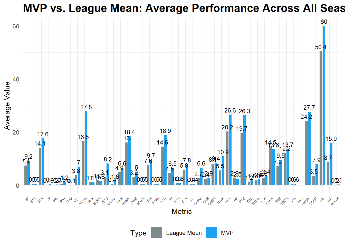
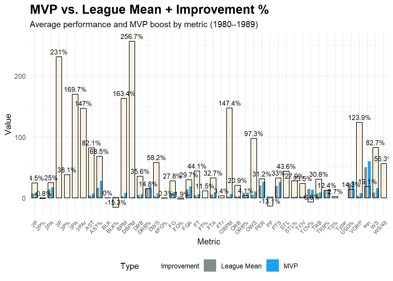
## 1980-1989赛季:
```{r}
library(readxl)
library(dplyr)
library(tidyr)
library(ggplot2)
library(stringr)

# 读取数据
df <- read_excel("C:/Users/86133/Desktop/object/MVP/MVP_Mean/MVP_mean_1980_89.xlsx", sheet = "Sheet1")

# 提取年份和类型
df <- df %>%
  mutate(
    Season = str_extract(name, "\\d{4}"),
    Type = ifelse(grepl("Mean", name), "League Mean", "MVP")
  )

# 分别计算平均值(跨所有赛季)
mvp_mean <- df %>%
  filter(Type == "MVP") %>%
  select(-name, -Season) %>%
  summarise(across(everything(), mean, na.rm = TRUE)) %>%
  pivot_longer(cols = everything(), names_to = "Metric", values_to = "Value") %>%
  mutate(Type = "MVP")

league_mean <- df %>%
  filter(Type == "League Mean") %>%
  select(-name, -Season) %>%
  summarise(across(everything(), mean, na.rm = TRUE)) %>%
  pivot_longer(cols = everything(), names_to = "Metric", values_to = "Value") %>%
  mutate(Type = "League Mean")

# 合并
compare_df <- bind_rows(mvp_mean, league_mean)

# 绘图
ggplot(compare_df, aes(x = Metric, y = Value, fill = Type)) +
  geom_col(position = position_dodge(width = 0.8), width = 0.7) +
  geom_text(
    aes(label = round(Value, 1)),
    position = position_dodge(width = 0.8),
    vjust = -0.5,
    size = 3
  ) +
  scale_fill_manual(values = c("MVP" = "#1DA1F2", "League Mean" = "#7F8C8D")) +
  labs(
    title = "MVP vs. League Mean: Average Performance Across All Seasons",
    x = "Metric",
    y = "Average Value",
    fill = "Type"
  ) +
  theme_minimal() +
  theme(
    axis.text.x = element_text(angle = 45, hjust = 1,size=5),
    plot.title = element_text(size = 16, face = "bold"),
    legend.position = "bottom"
  )
```
```{r}
#| warning: false
#| # 读取数据
df <- read_excel("C:/Users/86133/Desktop/object/MVP/MVP_Mean/MVP_mean_1980_89.xlsx", sheet = "Sheet1")

# 提取年份和类型
df <- df %>%
  mutate(
    Season = str_extract(name, "\\d{4}"),
    Type = ifelse(grepl("Mean", name), "League Mean", "MVP")
  )

# 分别计算平均值(跨所有赛季)
mvp_mean <- df %>%
  filter(Type == "MVP") %>%
  select(-name, -Season) %>%
  summarise(across(everything(), mean, na.rm = TRUE)) %>%
  pivot_longer(cols = everything(), names_to = "Metric", values_to = "Value") %>%
  mutate(Type = "MVP")

league_mean <- df %>%
  filter(Type == "League Mean") %>%
  select(-name, -Season) %>%
  summarise(across(everything(), mean, na.rm = TRUE)) %>%
  pivot_longer(cols = everything(), names_to = "Metric", values_to = "Value") %>%
  mutate(Type = "League Mean")

# 合并
compare_df <- bind_rows(mvp_mean, league_mean)
# 将 MVP 和 League Mean 数据展开为宽格式
df_wide <- compare_df %>%
  pivot_wider(names_from = Type, values_from = Value)

# 计算提升百分比(%),并构建新数据框
improvement_df <- df_wide %>%
  mutate(`Improvement %` = (`MVP` - `League Mean`) / `League Mean` * 100) %>%
  select(Metric, `Improvement %`) %>%
  mutate(Type = "Improvement") %>%
  rename(Value = `Improvement %`)

compare_all <- bind_rows(compare_df, improvement_df)

library(ggplot2)

ggplot(compare_all, aes(x = Metric, y = Value, fill = Type)) +
  geom_col(
    data = subset(compare_all, Type != "Improvement"),
    position = position_dodge(width = 0.9),
    width = 0.7
  ) +
  geom_col(
    data = subset(compare_all, Type == "Improvement"),
    aes(fill = "Improvement"),
    position = position_dodge(width = 0.9),
    width = 0.7,
    color = "black",
    fill = "orange",
    alpha = 0.1
  ) +
  geom_text(
    data = subset(compare_all, Type == "Improvement"),
    aes(label = paste0(round(Value, 1), "%")),
    vjust = -0.5,
    size = 3,
    position = position_dodge(width = 0.9)
  ) +
  scale_fill_manual(
    values = c("Improvement" = "orange","MVP" = "#1DA1F2", "League Mean" = "#7F8C8D")
  ) +
  labs(
    title = "MVP vs. League Mean + Improvement %",
    subtitle = "Average performance and MVP boost by metric (1980–1989)",
    x = "Metric",
    y = "Value",
    fill = "Type"
  ) +
  theme_minimal() +
  theme(
    axis.text.x = element_text(angle = 45, hjust = 1,size=7),
    plot.title = element_text(size = 16, face = "bold"),
    legend.position = "bottom"
  )
```